Introduction
Excel is the fastest way to calculate percentages for marks, sales, budgets and reports. Once you know the percentage formula in Excel, you can work out hundreds of results in seconds instead of using a calculator one by one.
This guide shows you the basic formula, how to format results as percentages, and nine practical examples you can copy into your own sheets.
- Excel stores percentages as decimals.
- The % format multiplies the value by 100 for display.
- One formula can be copied down a whole column.
Table of Contents
What Is the Percentage Formula in Excel?
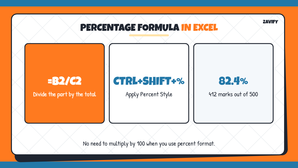
The basic percentage formula in Excel is =Part/Total. You divide the part by the total and then apply the Percent Style format. For example, if marks obtained are in B2 and maximum marks are in C2, the formula is =B2/C2.
You do not need to multiply by 100 when you use percentage formatting. Excel does that for display automatically.
- Part: the value you want as a percentage.
- Total: the whole amount.
- Format: Percent Style (Ctrl + Shift + %).
How Does the Percentage Formula in Excel Work?
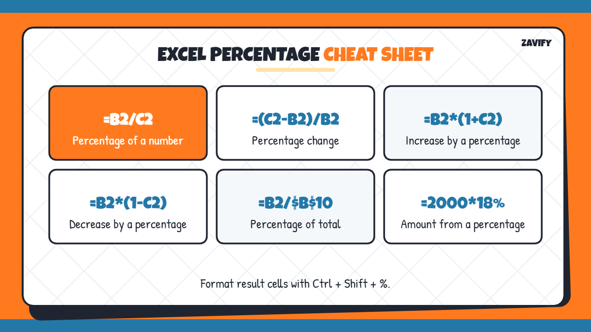
Here are the most common versions of the percentage formula in Excel at a glance:
| Task | Formula | Example Result |
|---|---|---|
| Percentage of a number | =B2/C2 | 412/500 = 82.4% |
| Percentage change | =(C2-B2)/B2 | 50,000 to 62,000 = 24% |
| Increase by a percentage | =B2*(1+C2) | 25,000 + 10% = 27,500 |
| Decrease by a percentage | =B2*(1-C2) | 1,500 − 20% = 1,200 |
| Percentage of total | =B2/$B$10 | Share of a column total |
Let us now go through each method step by step.
1. Calculate the Percentage of Marks
Put marks obtained in column B and maximum marks in column C. In D2, type =B2/C2 and press Enter. For 412 out of 500, Excel shows 0.824, which becomes 82.4% after formatting. If your result is in CGPA instead, use our CGPA to percentage converter.
2. Format the Result as a Percentage
Select the result cells and press Ctrl + Shift + %, or click the % button on the Home tab. Use the Increase Decimal button to show 82.40% instead of 82%.
- Format first, then type values like 25 to get 25%.
- Use two decimals for marks and reports.
3. Copy the Formula Down the Column
Drag the small fill handle at the bottom-right of D2 down the column. Excel adjusts the percentage formula in Excel for each row automatically, so every student gets the correct result.
4. Find the Percentage of a Total
To see what share each item is of a total, lock the total cell with dollar signs: =B2/$B$10. The $ signs keep B10 fixed when you copy the formula down.
5. Calculate Percentage Change
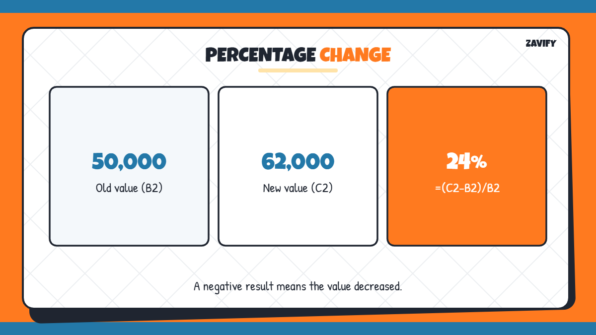
To measure growth or decline between two values, use =(New-Old)/Old. If sales rose from 50,000 in B2 to 62,000 in C2, the formula =(C2-B2)/B2 gives 24%. A negative result shows a decrease.
6. Increase a Number by a Percentage
To add a percentage, use =Value*(1+Percent). A salary of 25,000 with a 10% hike in C2 becomes =B2*(1+C2) = 27,500.
7. Decrease a Number by a Percentage
For discounts, use =Value*(1-Percent). A price of 1,500 with a 20% discount becomes =B2*(1-C2) = 1,200.
8. Find the Amount From a Percentage
To find what a percentage of a number is, multiply them. For 18% of 2,000, type =2000*18% to get 360. This version of the percentage formula in Excel is useful for GST, commissions and tips.
9. Find the Total From a Part and Percentage
If you know a part and its percentage, divide: =Part/Percent. If 360 is 18% of a number, =360/18% returns 2,000.
Add Grades With the IF Function
Once you have the percentage, you can add a grade or result column. If the percentage is in D2, the formula =IF(D2>=33%,”Pass”,”Fail”) shows Pass or Fail instantly. For several grades, nest IF functions or use IFS, for example =IFS(D2>=90%,”A+”,D2>=75%,”A”,D2>=60%,”B”,TRUE,”C”). Combining the percentage formula in Excel with IF saves hours when preparing class results.
- Change the cut-off values to match your board or school rules.
- Use conditional formatting to colour failing rows red.
Build a Simple Percentage Marksheet
A clean marksheet layout makes the formulas easy to manage. Put student names in column A, marks obtained in column B, maximum marks in column C, the percentage in column D, and the grade in column E. Freeze the header row with View → Freeze Panes so the column titles stay visible while you scroll.
Finally, add a summary row at the bottom. Use =AVERAGE(D2:D41) for the class average percentage, =MAX(D2:D41) for the highest score and =COUNTIF(E2:E41,”Pass”) to count how many students passed. This turns a basic percentage formula in Excel into a complete result sheet.
Show Percentages in a Chart
Charts make percentages easier to understand at a glance. Select your names and percentage columns, go to Insert, and choose a column or pie chart. Pie charts work well for a share of a total, while column charts are better for comparing students or months.
Using the Percentage Formula in Google Sheets
The same percentage formula in Excel works in Google Sheets. Type =B2/C2, then choose Format → Number → Percent. Shortcuts and the fill handle work the same way.
Common Mistakes With the Percentage Formula in Excel
Even simple formulas can give wrong results if you miss these points:
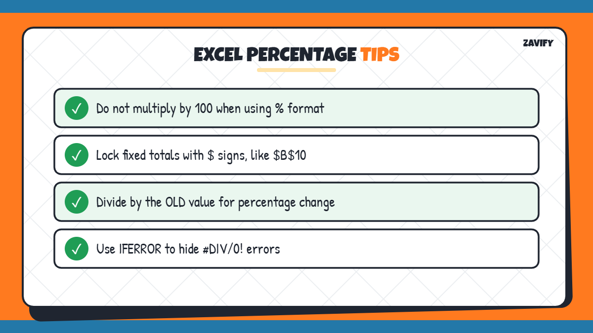
- Multiplying by 100 and then applying % format, which shows 8240%.
- Forgetting $ signs when dividing by a fixed total.
- Dividing by the new value instead of the old one for percentage change.
- Typing percentages as whole numbers in general-format cells.
- Dividing by an empty cell, which causes a #DIV/0! error.
Frequently Asked Questions
What is the percentage formula in Excel?
The basic percentage formula in Excel is =Part/Total, followed by Percent Style formatting.
How do I calculate percentage in Excel for marks?
Divide marks obtained by maximum marks, for example =B2/C2, and format the cell as a percentage.
How do I calculate percentage increase in Excel?
Use =(New-Old)/Old and format the result as a percentage.
Why does Excel show 8240% instead of 82.4%?
You probably multiplied by 100 and also applied percentage format. Remove the ×100 from the formula.
How do I fix the #DIV/0! error?
It appears when the total cell is empty or zero. Use =IFERROR(B2/C2,””) to hide the error.
Conclusion
The percentage formula in Excel is simple: divide the part by the total and apply percentage formatting. With small changes, the same idea handles percentage change, increases, discounts and shares of a total.
Practise these nine examples on a sample sheet, save it as a template, and you will be able to calculate percentages for marks, budgets and reports in seconds.